38 data labels excel 2013
How to Add Data Labels in Excel - Excelchat | Excelchat How to Add Data Labels In Excel 2013 And Later Versions In Excel 2013 and the later versions we need to do the followings; Click anywhere in the chart area to display the Chart Elements button Figure 5. Chart Elements Button Click the Chart Elements button > Select the Data Labels, then click the Arrow to choose the data labels position. Figure 6. How to Customize Chart Elements in Excel 2013 - dummies To add data labels to your selected chart and position them, click the Chart Elements button next to the chart and then select the Data Labels check box before you select one of the following options on its continuation menu: Center to position the data labels in the middle of each data point. Inside End to position the data labels inside each ...
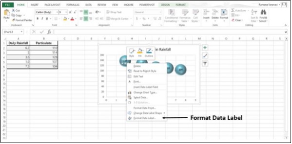
Values From Cell: Missing Data Labels Option in Excel 2013 ... A couple articles refer to formatting data labels and values to have it pull what you want. I have a feeling they used a 3rd party ad-in like tech-cell or some such and because I don't have the add in its not happy. Im following the blog reference here: Adding rich data labels to charts in Excel 2013 - Office Blogs
Data labels excel 2013
Excel 2013 - Line Chart Data Labels - Data Callout submenu ... In one of them I can see the Data Callout submenu which allows me to specific content for data labels to appear at specific points on the line-graph. The "label options/label contains" area in the formatting box then includes a "value from cells" tickbox that allows me specify that the values that come from a specific excel cell range. Values From Cell: Missing Data Labels Option in Excel 2013? When a chart created in 2013 using the "Values from Cell" data label option is opened with any earlier version of Excel, the data labels will show as " [CELLRANGE]". If you want to ensure that data labels survive different generations of Excel, you need to revert to the old technique: Insert data labels Edit each individual data label Change the format of data labels in a chart To get there, after adding your data labels, select the data label to format, and then click Chart Elements > Data Labels > More Options. To go to the appropriate area, click one of the four icons ( Fill & Line, Effects, Size & Properties ( Layout & Properties in Outlook or Word), or Label Options) shown here.
Data labels excel 2013. How to Data Labels in a Line Graph in Excel 2013 - YouTube Want to insert Data Labels in a line graph in Microsoft® Excel 2013? Follow the easy steps shown in this video. Content in this video is provided on an ""as ... Change the format of data labels in a chart To get there, after adding your data labels, select the data label to format, and then click Chart Elements > Data Labels > More Options. To go to the appropriate area, click one of the four icons ( Fill & Line, Effects, Size & Properties ( Layout & Properties in Outlook or Word), or Label Options) shown here. How to Add Data Labels to your Excel Chart in Excel 2013 ... Data labels show the values next to the corresponding chart element, for instance a percentage next to a piece from a pie chart, or a total value next to a column in a column chart. You can choose... How to insert data labels to a Pie chart in Excel 2013 ... This video will show you the simple steps to insert Data Labels in a pie chart in Microsoft® Excel 2013. Content in this video is provided on an "as is" basi...
Edit titles or data labels in a chart - support.microsoft.com The first click selects the data labels for the whole data series, and the second click selects the individual data label. Right-click the data label, and then click Format Data Label or Format Data Labels. Click Label Options if it's not selected, and then select the Reset Label Text check box. Top of Page How-to Use Data Labels from a Range in an Excel Chart 1) Create Chart Data Range and Data Label Range. First we need to create two (2) different data ranges in our Excel Spreadsheet. · 2) Create Chart. Now we are ... Creating a chart with dynamic labels - Microsoft Excel 2013 Excel 2013 365 2016 This tip shows how to create dynamically updated chart labels that depend on value or other cells. The trick of this chart is to show data from specific cells in the chart labels. How to Add Axis Labels in Excel 2013 - YouTube How to Add Axis Labels in Excel 2013For more tips and tricks, be sure to check out is a tutorial on how to add axis labels in E...
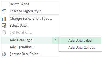
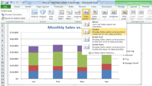
How to Data Labels in a Bar Graph in Excel 2013 - YouTube Watch this video to know about the steps to add data labels to a Bar Graph in Microsoft® Excel 2013. To access expert tech support, call iYogi™ at toll-free ... How to add data labels from different column in an Excel ... Right click the data series in the chart, and select Add Data Labels > Add Data Labels from the context menu to add data labels. 2. Click any data label to select all data labels, and then click the specified data label to select it only in the chart. 3. Add a Data Callout Label to Charts in Excel 2013 ... In the upper right corner, next to your chart, click the Chart Elements button (plus sign), and then click Data Labels. A right pointing arrow will appear, click on this arrow to view the submenu. Select Data Callout. Once the Data Callout Labels have been added, you can re-position them by clicking on their borders and dragging to a new position. Move data labels - support.microsoft.com Right-click the selection > Chart Elements > Data Labels arrow, and select the placement option you want. Different options are available for different chart types. For example, you can place data labels outside of the data points in a pie chart but not in a column chart.
Creating a chart with dynamic labels - Microsoft Excel 2013
Custom Data Labels with Colors and Symbols in Excel Charts ... The basic idea behind custom label is to connect each data label to certain cell in the Excel worksheet and so whatever goes in that cell will appear on the chart as data label. So once a data label is connected to a cell, we apply custom number formatting on the cell and the results will show up on chart also.

Microsoft Excel Tutorials: The Chart Layout Panels
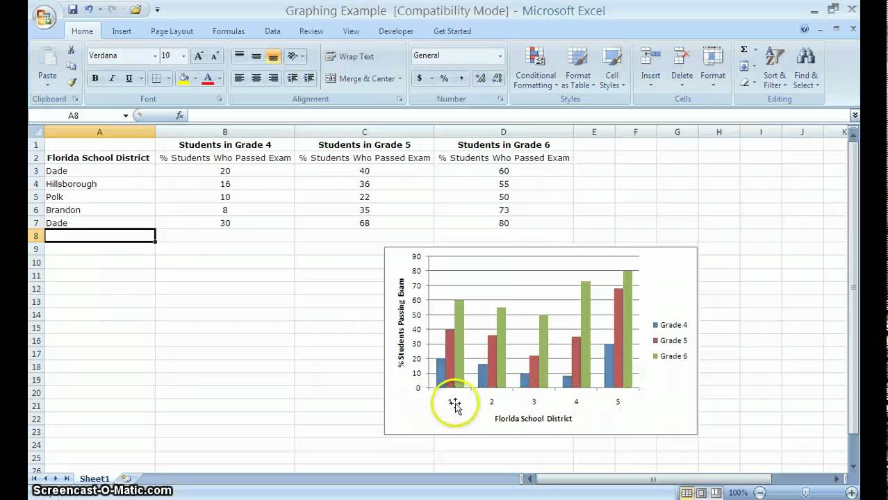
Excel Tips n Tricks -Tip 8 (Applying Chart Data Labels ... Click on the plus symbol, the first icon, and check "Data Labels". Now you will see them added to your chart. You can also click on the right arrow on "Data Labels" and select where you want the data labels to be aligned, in other words center, right, top, bottom and so on. Picture 4 4. I modified the chart and axis titles to look good.

Show Trend Arrows in Excel Chart Data Labels
formatting - How to format Microsoft Excel data labels ... To get this to work, I formatted the cell's of the data column 4 4 4 4 3.5 13.5, by either selecting the column and then right click and format cells or by right clicking on the chart and selecting format data labels.I formatted this with the regular expression $#K so that the data then shows as $4K $4K $4K $4K $4K $14K. The consequence is that the number is rounded to not include the decimal.

Create Custom Data Labels in Excel Charts - YouTube
Apply Custom Data Labels to Charted Points - Peltier Tech For data labels, the best tool by far is the XY chart label add in. I have Excel 2013 and have found that the Excel linked labels are not as reliable when the cells change as Rob Bovey's add in. Excel is complicated enough. We don't need to add complexity. Cheers,
Advanced Excel - Краткое руководство - CoderLessons.com
How to Print Labels from Excel - Lifewire These instructions apply to Excel and Word 2019, 2016, and 2013 and Excel and Word for Microsoft 365. How to Print Labels From Excel You can print mailing labels from Excel in a matter of minutes using the mail merge feature in Word.

Enable or Disable Excel Data Labels at the click of a button - How To - PakAccountants.com
Adding Data Labels to Your Chart (Microsoft Excel) To add data labels in Excel 2013 or Excel 2016, follow these steps: Activate the chart by clicking on it, if necessary. Make sure the Design tab of the ribbon is displayed. (This will appear when the chart is selected.) Click the Add Chart Element drop-down list. Select the Data Labels tool.
How to Change X axis Categories - YouTube
Adding rich data labels to charts in Excel 2013 - Microsoft You can do this by adjusting the zoom control on the bottom right corner of Excel's chrome. Then, select the value in the data label and hit the right-arrow key on your keyboard. The story behind the data in our example is that the temperature increased significantly on Wednesday and that appeared to help drive up business at the lemonade stand.

Chart Data Labels in PowerPoint 2011 for Mac
Add or remove data labels in a chart Right-click the data series or data label to display more data for, and then click Format Data Labels. Click Label Options and under Label Contains, select the Values From Cells checkbox. When the Data Label Range dialog box appears, go back to the spreadsheet and select the range for which you want the cell values to display as data labels.
How to Add Data Labels in Excel - Excelchat | Excelchat
Change the format of data labels in a chart To get there, after adding your data labels, select the data label to format, and then click Chart Elements > Data Labels > More Options. To go to the appropriate area, click one of the four icons ( Fill & Line, Effects, Size & Properties ( Layout & Properties in Outlook or Word), or Label Options) shown here.
Format Number Options for Chart Data Labels in Excel 2011 for Mac
Values From Cell: Missing Data Labels Option in Excel 2013? When a chart created in 2013 using the "Values from Cell" data label option is opened with any earlier version of Excel, the data labels will show as " [CELLRANGE]". If you want to ensure that data labels survive different generations of Excel, you need to revert to the old technique: Insert data labels Edit each individual data label

34 How To Add Label To Excel Chart
Excel 2013 - Line Chart Data Labels - Data Callout submenu ... In one of them I can see the Data Callout submenu which allows me to specific content for data labels to appear at specific points on the line-graph. The "label options/label contains" area in the formatting box then includes a "value from cells" tickbox that allows me specify that the values that come from a specific excel cell range.
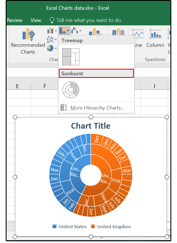
What to do with Excel 2016's new chart styles: Treemap, Sunburst, and Box & Whisker | PCWorld
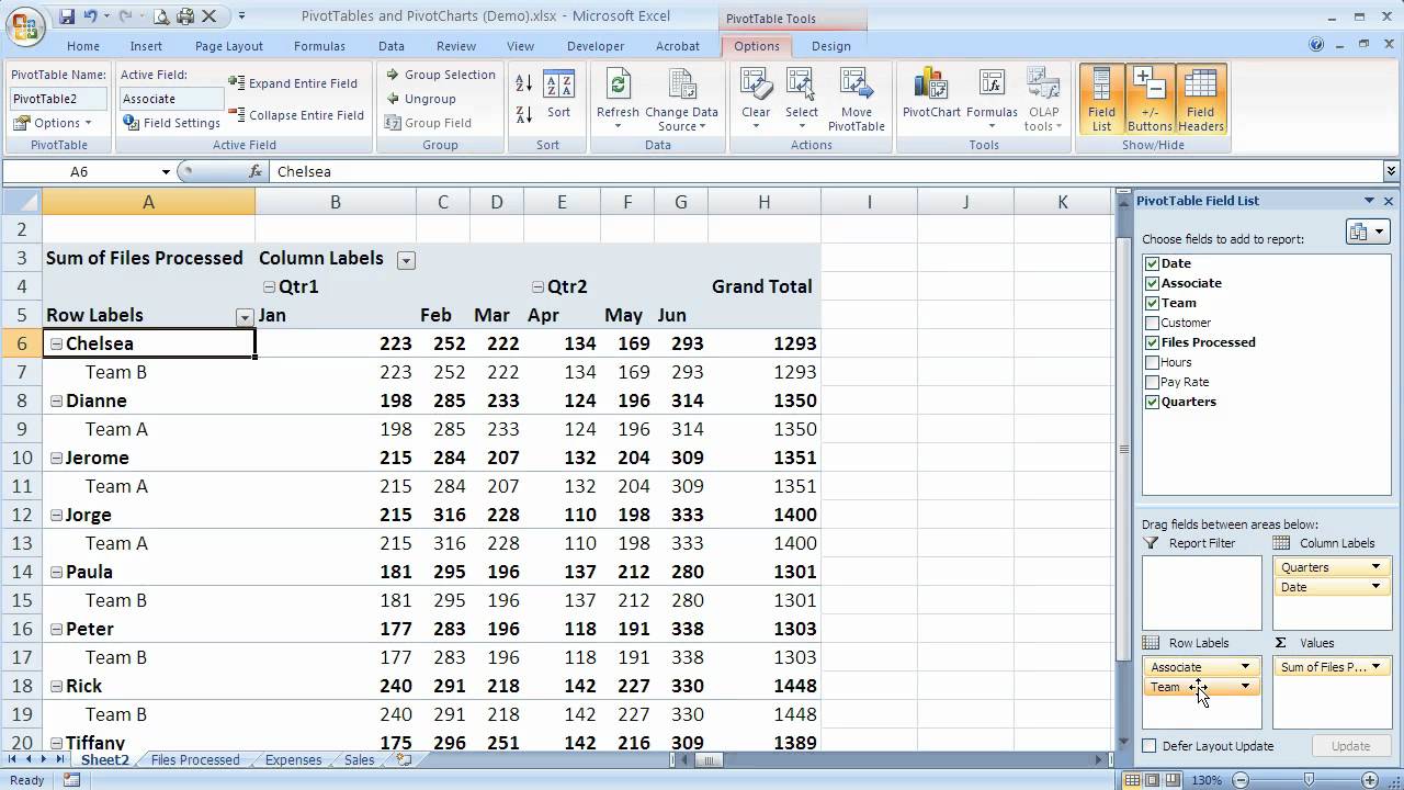
How to group row labels in Excel 2007 PivotTables (Excel 07-104) - YouTube

Automatically update data labels on Excel chart (Excel 2016) - Stack Overflow

Callout Data Labels for Charts in PowerPoint 2013 for Windows
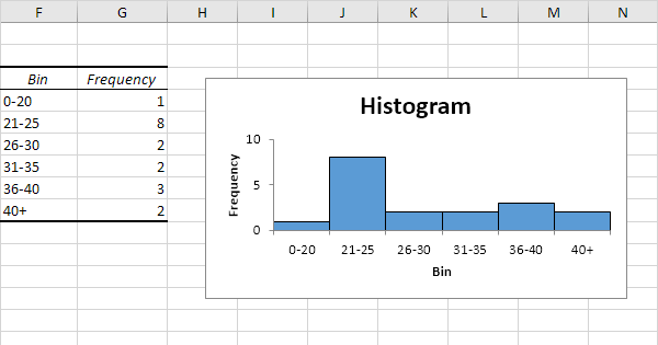
Histogram in Excel - Easy Excel Tutorial
Excel 2013 - Manually adding multiple data sets to scatter plot - YouTube

Printing in Excel 7 - Repeat Row & Column Titles on Every Printed Page from Excel - Page Setup ...
Post a Comment for "38 data labels excel 2013"