44 how to display data labels above the columns in excel
EOF Excel Pivot values as column labels - Stack Overflow If you have Excel for Office 365 (or Excel 2021) with the FILTER function, you can use the following: Note that I used a table with structured references for the data source. This has advantages in editing the table in the future. For "pivot" header: =TRANSPOSE(SORT(UNIQUE(Table1[Country]))) For the columns:
How to mail merge and print labels from Excel - Ablebits Select document type. The Mail Merge pane will open in the right part of the screen. In the first step of the wizard, you select Labels and click Next: Starting document near the bottom. (Or you can go to the Mailings tab > Start Mail Merge group and click Start Mail Merge > Labels .) Choose the starting document.

How to display data labels above the columns in excel
How to Add Labels to Scatterplot Points in Excel - Statology Step 3: Add Labels to Points. Next, click anywhere on the chart until a green plus (+) sign appears in the top right corner. Then click Data Labels, then click More Options…. In the Format Data Labels window that appears on the right of the screen, uncheck the box next to Y Value and check the box next to Value From Cells. Data labels on secondary axis position - Microsoft Tech Community Bars on the primary axis are stacked. But secondary axis bars are Clustered - Since the secondary axis is not stacked, why can't the labels be on the outside end? If I make a Column Graph, I am able to choose Outside End for the secondary axis (when the primary axis is stacked). I can't figure out how to beat this with VBA code either. Help ... 5 New Charts to Visually Display Data in Excel 2019 - dummies Enter the labels and data. Put them in the order you want them to appear in the chart, from top to bottom. You can convert the range to a table to sort it more easily. Select the labels and data and then click Insert → Insert Waterfall, Funnel, Stock, Surface, or Radar Chart → Funnel. Format the chart as desired.
How to display data labels above the columns in excel. 38 how to show data labels as percentage in excel Add percentages in stacked column chart 1. Select data range you need and click Insert > Column > Stacked Column. See screenshot: 2. Click at the column and then click Design > Switch Row/Column. 3. In Excel 2007, click Layout > Data Labels > Center . In Excel 2013 or the new version, click Design > Add Chart Element > Data Labels > Center. 4. 3 Ways to Transpose Data Horizontally in Excel - MUO 1. Simple Copy Pasting. This is a straightforward way to transpose vertical rows into horizontal columns by copying the data in rows and pasting it into columns. Here is how you can transpose data using this method. 1. Select the cells you want to transpose. 2. Press CTRL + C to copy it. 3. Excel Conditional Formatting Data Bars On the Ribbon, click the Home tab, and then in the Styles group, click Conditional Formatting. In the list of conditional formatting options, click Data Bars, and then click one of the Data Bar options -- Gradient Fill or Solid Fill. (see tips below) The selected cells now show Data Bars, along with the original numbers. How to See Headings and Row Labels as You Scroll Around a Report 1. Select cell G6. This is the first non-frozen cell. 2. Select View, Freeze Panes, Freeze Panes. You will see a solid line between columns F and G and between rows 5 and 6. Results: As you scroll, you can always see the headings. Figure 65. Scroll out to October and you can still see A:F.
Headings Missing in Excel: How to Show Row Numbers & Column Letters! How to get missing row numbers and column letters back. Follow these two steps to show row and column headings: If the column letters and row numbers are missing, go to View and click on "Headings". In order to show (or hide) the row and column numbers and letters go to the View ribbon. Set the check mark at "Headings". Guide: How to Name Column in Excel | Indeed.com Select "Define Name" under the Defined Names group in the Ribbon to open the New Name window. Enter your new column name in the text box. Click the "Scope" drop-down menu and then "Workbook" to apply the change to all the sheets. 5. Clean all column names. Custom Chart Data Labels In Excel With Formulas Follow the steps below to create the custom data labels. Select the chart label you want to change. In the formula-bar hit = (equals), select the cell reference containing your chart label's data. In this case, the first label is in cell E2. Finally, repeat for all your chart laebls. How can I get data labels to show for each column in a bar chart? Hi @knizefl . Turn on 'Overflow text' under Data label' Format tab. Also, you can adjust the position of the Data Label by switching to 'Outside End' or 'Inside Center' so that your Data Label gets displayed properly. If this post helps, then mark it as 'Accept as Solution ' so that it could help others. Regards,
Excel 365 multiple columns with data, but all mixed up. How to sort so ... So I have an excel document that contains information on various software names and types, having used Text to Columns I have unsorted data running left to right that is not alphabetical. the row above and below will hold different data in the same cell. How can I sort several columns - up to 15 to display each title in the same column? 5 New Charts to Visually Display Data in Excel 2019 - dummies Enter the labels and data. Put them in the order you want them to appear in the chart, from top to bottom. You can convert the range to a table to sort it more easily. Select the labels and data and then click Insert → Insert Waterfall, Funnel, Stock, Surface, or Radar Chart → Funnel. Format the chart as desired. Data labels on secondary axis position - Microsoft Tech Community Bars on the primary axis are stacked. But secondary axis bars are Clustered - Since the secondary axis is not stacked, why can't the labels be on the outside end? If I make a Column Graph, I am able to choose Outside End for the secondary axis (when the primary axis is stacked). I can't figure out how to beat this with VBA code either. Help ... How to Add Labels to Scatterplot Points in Excel - Statology Step 3: Add Labels to Points. Next, click anywhere on the chart until a green plus (+) sign appears in the top right corner. Then click Data Labels, then click More Options…. In the Format Data Labels window that appears on the right of the screen, uncheck the box next to Y Value and check the box next to Value From Cells.

Excel Dashboard Templates How-to Use Data Labels from a Range in an Excel Chart - Excel ...
Creating a chart

How to plot stacked columns with Excel
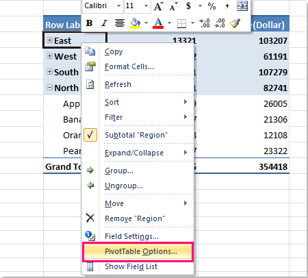
How to hide expand collapse buttons in pivot table?

Adobe Using RoboHelp (2017 Release) Robo Help 2017 User Guide Ug En

Advanced Excel Charts: What to Know to Take Your Charts Up a Notch – ZingUrl.com
How to Show Recessions in Excel Charts - ExcelUser.com

PPC Storytelling: How to Make an Excel Bubble Chart for PPC - Business 2 Community
Post a Comment for "44 how to display data labels above the columns in excel"