39 excel chart add data labels
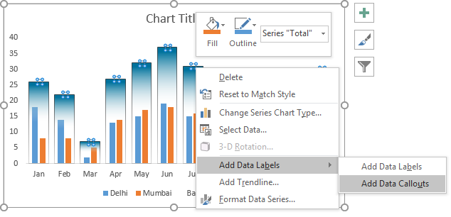
How to add total labels to stacked column chart in Excel? - ExtendOffice Select and right click the new line chart and choose Add Data Labels > Add Data Labels from the right-clicking menu. See screenshot: And now each label has been added to corresponding data point of the Total data series. And the data labels stay at upper-right corners of each column. 5. Add a DATA LABEL to ONE POINT on a chart in Excel Steps shown in the video above: Click on the chart line to add the data point to. All the data points will be highlighted. Click again on the single point that you want to add a data label to. Right-click and select ' Add data label ' This is the key step! Right-click again on the data point itself (not the label) and select ' Format data label '.
How to add or move data labels in Excel chart? - ExtendOffice To add or move data labels in a chart, you can do as below steps: In Excel 2013 or 2016. 1. Click the chart to show the Chart Elements button .. 2. Then click the Chart Elements, and check Data Labels, then you can click the arrow to choose an option about the data labels in the sub menu.See screenshot:
Excel chart add data labels
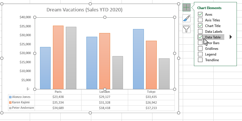
Excel charts: how to move data labels to legend @Matt_Fischer-Daly . You can't do that, but you can show a data table below the chart instead of data labels: Click anywhere on the chart. On the Design tab of the ribbon (under Chart Tools), in the Chart Layouts group, click Add Chart Element > Data Table > With Legend Keys (or No Legend Keys if you prefer) Excel Chart Tutorial: a Beginner's Step-By-Step Guide Sure, the numbers themselves show impressive growth, and she could simply spit out those digits during her presentation. But, she really wants to make an impact—so, she’s going to use an Excel chart to display the subscriber growth she’s worked so hard for. How to build an Excel chart: A step-by-step Excel chart tutorial 1. Get your data ... How to Add Data Labels in Excel - Excelchat | Excelchat After inserting a chart in Excel 2010 and earlier versions we need to do the followings to add data labels to the chart; Click inside the chart area to display the Chart Tools. Figure 2. Chart Tools Click on Layout tab of the Chart Tools. In Labels group, click on Data Labels and select the position to add labels to the chart. Figure 3.
Excel chart add data labels. 100% Stacked Area Chart: Product mix over time | Exceljet How to create this chart. Select the data and select line chart on the ribbon: Select the 100% Stacked Area option under 2d area. Chart as inserted. Select and delete legend. Add data labels to chart: Select each data series. Check Series Name, then uncheck Value: Final 100% Stacked Area chart before title and size changes: How To Add Data Labels In Excel - newall.northminster.info To do this, click the "format" tab within the "chart tools" contextual tab in the ribbon. Use the following steps to add data labels to series in a chart: Source: pakaccountants.com. Add custom data labels from the column "x axis labels". In this second method, we will add the x and y axis labels in excel by chart element button. Custom Chart Data Labels In Excel With Formulas Follow the steps below to create the custom data labels. Select the chart label you want to change. In the formula-bar hit = (equals), select the cell reference containing your chart label's data. In this case, the first label is in cell E2. Finally, repeat for all your chart laebls. How to add data labels from different column in an Excel chart? This method will guide you to manually add a data label from a cell of different column at a time in an Excel chart. 1. Right click the data series in the chart, and select Add Data Labels > Add Data Labels from the context menu to add data labels. 2. Click any data label to select all data labels, and then click the specified data label to ...
Change the format of data labels in a chart To get there, after adding your data labels, select the data label to format, and then click Chart Elements > Data Labels > More Options. To go to the appropriate area, click one of the four icons ( Fill & Line, Effects, Size & Properties ( Layout & Properties in Outlook or Word), or Label Options) shown here. How to Make a Pie Chart in Excel & Add Rich Data Labels to ... Creating and formatting the Pie Chart. 1) Select the data. 2) Go to Insert> Charts> click on the drop-down arrow next to Pie Chart and under 2-D Pie, select the Pie Chart, shown below. 3) Chang the chart title to Breakdown of Errors Made During the Match, by clicking on it and typing the new title. Excel: How to Create a Bubble Chart with Labels - Statology Step 3: Add Labels. To add labels to the bubble chart, click anywhere on the chart and then click the green plus "+" sign in the top right corner. Then click the arrow next to Data Labels and then click More Options in the dropdown menu: In the panel that appears on the right side of the screen, check the box next to Value From Cells within ... How to Add Data Labels to Scatter Plot in Excel (2 Easy Ways) - ExcelDemy At first, go to the sheet Chart Elements. Then, select the Scatter Plot already inserted. After that, go to the Chart Design tab. Later, select Add Chart Element > Data Labels > None. This is how we can remove the data labels. Read More: Use Scatter Chart in Excel to Find Relationships between Two Data Series. 2.
Prevent Overlapping Data Labels in Excel Charts - Peltier Tech May 24, 2021 · Here is the chart after running the routine, without allowing any overlap between labels (OverlapTolerance = zero).All labels can be read, but the space between them is greater than needed (you could almost stick another label between any two adjacent labels here), and some labels have moved far from the points they label. Add or remove data labels in a chart - support.microsoft.com Depending on what you want to highlight on a chart, you can add labels to one series, all the series (the whole chart), or one data point. Add data labels. You can add data labels to show the data point values from the Excel sheet in the chart. This step applies to Word for Mac only: On the View menu, click Print Layout. How to create Custom Data Labels in Excel Charts - Efficiency 365 Create the chart as usual. Add default data labels. Click on each unwanted label (using slow double click) and delete it. Select each item where you want the custom label one at a time. Press F2 to move focus to the Formula editing box. Type the equal to sign. Now click on the cell which contains the appropriate label. How to Add Two Data Labels in Excel Chart (with Easy Steps) Select the data labels. Then right-click your mouse to bring the menu. Format Data Labels side-bar will appear. You will see many options available there. Check Category Name. Your chart will look like this. Now you can see the category and value in data labels. Read More: How to Format Data Labels in Excel (with Easy Steps) Things to Remember
Creative Column Chart that Includes Totals in Excel
Add or remove data labels in a chart - support.microsoft.com Add data labels to a chart Click the data series or chart. To label one data point, after clicking the series, click that data point. In the upper right corner, next to the chart, click Add Chart Element > Data Labels. To change the location, click the arrow, and choose an option.

How to Add Axis Labels to a Chart in Excel | CustomGuide
HOW TO CREATE A BAR CHART WITH LABELS INSIDE BARS IN EXCEL - simplexCT 7. In the chart, right-click the Series "# Footballers" Data Labels and then, on the short-cut menu, click Format Data Labels. 8. In the Format Data Labels pane, under Label Options selected, set the Label Position to Inside End. 9. Next, in the chart, select the Series 2 Data Labels and then set the Label Position to Inside Base.

Adding rich data labels to charts in Excel 2013 | Microsoft ...
Data Labels in Excel Pivot Chart (Detailed Analysis) 7 Suitable Examples with Data Labels in Excel Pivot Chart Considering All Factors 1. Adding Data Labels in Pivot Chart 2. Set Cell Values as Data Labels 3. Showing Percentages as Data Labels 4. Changing Appearance of Pivot Chart Labels 5. Changing Background of Data Labels 6. Dynamic Pivot Chart Data Labels with Slicers 7.

Add data labels and callouts to charts in Excel 365 ...
How to add data labels from different column in an Excel chart? Right click the data series in the chart, and select Add Data Labels > Add Data Labels from the context menu to add data labels. 2. Click any data label to select all data labels, and then click the specified data label to select it only in the chart. 3.
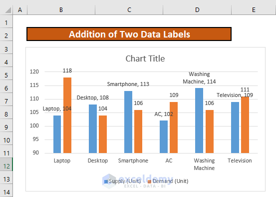
How to Add Two Data Labels in Excel Chart (with Easy Steps ...
Edit titles or data labels in a chart - support.microsoft.com On a chart, click one time or two times on the data label that you want to link to a corresponding worksheet cell. The first click selects the data labels for the whole data series, and the second click selects the individual data label. Right-click the data label, and then click Format Data Label or Format Data Labels.

How to add data labels from different column in an Excel chart?
How to Adjust Your Bar Chart’s Spacing in Microsoft Excel Jun 02, 2015 · In a line chart or a stacked line chart (a.k.a. stacked area chart), you can move the categories closer together by narrowing the graph. By default, Excel graphs are 3 inches tall and 5 inches wide. To nudge the categories closer together, you would adjust your graph so that it’s, let’s say, 3 inches tall and 4 inches wide.
How to Add Data Tables to a Chart in Excel - Business ...
Chart elements Excel not showing - profitclaims.com Chart Title. A chart title will add a small textbox to the top of your chart allowing you to name/label it. You can expand the checkbox to reveal locations for the chart title to be created at: Data Labels. Data labels can be added to show a value or percentage to a chart that otherwise might be too difficult to read off the chart.

How to Add Two Data Labels in Excel Chart (with Easy Steps ...
Create a multi-level category chart in Excel - ExtendOffice 22. Now the new series is shown as scatter dots and displayed on the right side of the plot area. Select the dots, click the Chart Elements button, and then check the Data Labels box. 23. Right click the data labels and select Format Data Labels from the right-clicking menu. 24. In the Format Data Labels pane, please do as follows.

how to add data labels into Excel graphs — storytelling with data
How to Use Cell Values for Excel Chart Labels - How-To Geek Mar 12, 2020 · Select the chart, choose the “Chart Elements” option, click the “Data Labels” arrow, and then “More Options.” Uncheck the “Value” box and check the “Value From Cells” box. Select cells C2:C6 to use for the data label range and then click the “OK” button.

Add or remove data labels in a chart
Excel.ChartDataLabels class - Office Add-ins | Microsoft Learn This connects the add-in's process to the Office host application's process. format. Specifies the format of chart data labels, which includes fill and font formatting. horizontal Alignment. Specifies the horizontal alignment for chart data label. See Excel.ChartTextHorizontalAlignment for details. This property is valid only when the ...

Excel charts: add title, customize chart axis, legend and ...
How to Add Data Labels in Excel - Excelchat | Excelchat After inserting a chart in Excel 2010 and earlier versions we need to do the followings to add data labels to the chart; Click inside the chart area to display the Chart Tools. Figure 2. Chart Tools Click on Layout tab of the Chart Tools. In Labels group, click on Data Labels and select the position to add labels to the chart. Figure 3.

Adding rich data labels to charts in Excel 2013 | Microsoft ...
Excel Chart Tutorial: a Beginner's Step-By-Step Guide Sure, the numbers themselves show impressive growth, and she could simply spit out those digits during her presentation. But, she really wants to make an impact—so, she’s going to use an Excel chart to display the subscriber growth she’s worked so hard for. How to build an Excel chart: A step-by-step Excel chart tutorial 1. Get your data ...

How to add data labels from different column in an Excel chart?
Excel charts: how to move data labels to legend @Matt_Fischer-Daly . You can't do that, but you can show a data table below the chart instead of data labels: Click anywhere on the chart. On the Design tab of the ribbon (under Chart Tools), in the Chart Layouts group, click Add Chart Element > Data Table > With Legend Keys (or No Legend Keys if you prefer)

Dynamically Label Excel Chart Series Lines • My Online ...

How to Change Excel Chart Data Labels to Custom Values?

Custom Data Labels with Colors and Symbols in Excel Charts ...

Is there a way to add data labels as percentages on the ...

How to Make a Pie Chart in Excel – Contextures Blog

Custom data labels in a chart
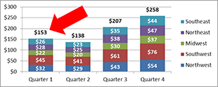
How to Add Totals to Stacked Charts for Readability - Excel ...

Add Total Values for Stacked Column and Stacked Bar Charts in ...

Excel charts: add title, customize chart axis, legend and ...

how to add data labels into Excel graphs — storytelling with data

microsoft excel - Adding data label only to the last value ...

How to Customize Your Excel Pivot Chart Data Labels - dummies

How to Add Data Labels in Excel - Excelchat | Excelchat

How to add total labels to stacked column chart in Excel?

Total of chart series – Excel kitchenette

Enable or Disable Excel Data Labels at the click of a button ...

Change the format of data labels in a chart

424 How to add data label to line chart in Excel 2016

How to Use Cell Values for Excel Chart Labels

Format Data Labels in Excel- Instructions - TeachUcomp, Inc.

microsoft excel - Adding data label only to the last value ...

Display Customized Data Labels on Charts & Graphs
Directly Labeling Excel Charts - PolicyViz

Apply Custom Data Labels to Charted Points - Peltier Tech

Chart Data Labels in PowerPoint 2011 for Mac
Example: Charts with Data Labels — XlsxWriter Documentation
Post a Comment for "39 excel chart add data labels"