45 adding chart labels in excel
Adding Data Labels to Your Chart (Microsoft Excel) - ExcelTips (ribbon) To add data labels in Excel 2013 or later versions, follow these steps: Activate the chart by clicking on it, if necessary. Make sure the Design tab of the ribbon is displayed. (This will appear when the chart is selected.) Click the Add Chart Element drop-down list. Select the Data Labels tool. How to Add Two Data Labels in Excel Chart (with Easy Steps) Table of Contents hide. Download Practice Workbook. 4 Quick Steps to Add Two Data Labels in Excel Chart. Step 1: Create a Chart to Represent Data. Step 2: Add 1st Data Label in Excel Chart. Step 3: Apply 2nd Data Label in Excel Chart. Step 4: Format Data Labels to Show Two Data Labels. Things to Remember.
How to Change Excel Chart Data Labels to Custom Values? 05.05.2010 · When you “add data labels” to a chart series, excel can show either “category” , “series” or “data point values” as data labels. But what if you want to have a data label that is altogether different, like this: You can change data labels and point them to different cells using this little trick. First add data labels to the chart (Layout Ribbon > Data Labels) Define the new ...

Adding chart labels in excel
How to Create Charts in Excel (In Easy Steps) - Excel Easy To move the legend to the right side of the chart, execute the following steps. 1. Select the chart. 2. Click the + button on the right side of the chart, click the arrow next to Legend and click Right. Result: Data Labels. You can use data labels to focus your readers' attention on a single data series or data point. 1. Select the chart. 2. Edit titles or data labels in a chart - support.microsoft.com On a chart, click one time or two times on the data label that you want to link to a corresponding worksheet cell. The first click selects the data labels for the whole data series, and the second click selects the individual data label. Right-click the data label, and then click Format Data Label or Format Data Labels. Add Excel Chart Labels. Adding Chart Labels in Excel. Excel ... - OzGrid With the above data, generate the chart below. First select the chart, then access the dialog below from the Chart Tools for Excel 1.1 toolbar / Charts / Add Labels. You may also access this tool by right-clicking on the chart and selecting Add Labels. The same dialog will appear.
Adding chart labels in excel. How To Add Data Labels In Excel - veganheath.info To get there, after adding your data labels, select the data label to format, and then click chart elements > data labels > more options. After picking the series, click the data point you want to label. Source: temotips.blogspot.com. Using excel chart element button to add axis labels. Click the chart to show the chart elements button. How to Add Data Labels to an Excel 2010 Chart - dummies Use the following steps to add data labels to series in a chart: Click anywhere on the chart that you want to modify. On the Chart Tools Layout tab, click the Data Labels button in the Labels group. None: The default choice; it means you don't want to display data labels. Center to position the data labels in the middle of each data point. Column Chart In Excel | How to insert 2-D Column Chart in Excel | add ... Column Chart In Excel | How to insert 2-D Column Chart in Excel | add Title, Legend, data labels EtcChannel PlaylistsPythonhttps:// ... Multiple Time Series in an Excel Chart - Peltier Tech 12.08.2016 · I recently showed several ways to display Multiple Series in One Excel Chart.The current article describes a special case of this, in which the X values are dates. Displaying multiple time series in an Excel chart is not difficult if all the series use the same dates, but it becomes a problem if the dates are different, for example, if the series show monthly and …
Column Chart with Primary and Secondary Axes - Peltier Tech 28.10.2013 · The second chart shows the plotted data for the X axis (column B) and data for the the two secondary series (blank and secondary, in columns E & F). I’ve added data labels above the bars with the series names, so you can see where the zero-height Blank bars are. The blanks in the first chart align with the bars in the second, and vice versa. How to ☝️Create a Run Chart in Excel [2 Free Templates] 17.07.2021 · Read more: How to Create a Gantt Chart in Excel. 2 Excel Run Chart Templates. Let’s face it. Chances are that you have too much stuff on your plate to build a run chart from the ground up. Luckily, we’ve got you covered! If you’re short on time, we’ve prepared two Excel run chart templates where everything has already been set up for you. How to add axis label to chart in Excel? - ExtendOffice Click to select the chart that you want to insert axis label. 2. Then click the Charts Elements button located the upper-right corner of the chart. In the expanded menu, check Axis Titles option, see screenshot: 3. And both the horizontal and vertical axis text boxes have been added to the chart, then click each of the axis text boxes and enter ... Adding Data Labels To An Excel Chart | MyExcelOnline In our example below, I add a Data Label to a column chart and then I format the data label using CTRL+1. I then select to custom format the numbers so it shows the values as thousands by adding a comma , after each zero and then showing the work k by adding "k". Example Custom Number Format: [$$-1004]#,##0 ,"k" ;- [$$-1004]#,##0 ,"k".
How to Make a Pie Chart in Excel & Add Rich Data Labels to 08.09.2022 · A pie chart is used to showcase parts of a whole or the proportions of a whole. There should be about five pieces in a pie chart if there are too many slices, then it’s best to use another type of chart or a pie of pie chart in order to showcase the data better. In this article, we are going to see a detailed description of how to make a pie chart in excel. Excel charts: add title, customize chart axis, legend and data labels Click the Chart Elements button, and select the Data Labels option. For example, this is how we can add labels to one of the data series in our Excel chart: For specific chart types, such as pie chart, you can also choose the labels location. For this, click the arrow next to Data Labels, and choose the option you want. How to Create a Dynamic Chart Range in Excel - Trump Excel This dynamic range is then used as the source data in a chart. As the data changes, the dynamic range updates instantly which leads to an update in the chart. Below is an example of a chart that uses a dynamic chart range. Note that the chart updates with the new data points for May and June as soon as the data in entered. how to add data labels into Excel graphs — storytelling with data There are a few different techniques we could use to create labels that look like this. Option 1: The "brute force" technique. The data labels for the two lines are not, technically, "data labels" at all. A text box was added to this graph, and then the numbers and category labels were simply typed in manually.
How-to Use Data Labels from a Range in an Excel Chart - Excel ...
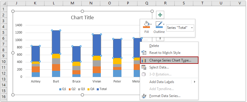
Adding rich data labels to charts in Excel 2013 One familiar and simple way is just single click on any data value (or column, in this example) to select the entire data series that it belongs to. Above, I have clicked all of the blue columns. Once the series is selected, I can right-click any column to pull up the context menu, then click the Add Data Labels entry.
How to add Axis Labels (X & Y) in Excel & Google Sheets ...
Change the format of data labels in a chart To get there, after adding your data labels, select the data label to format, and then click Chart Elements > Data Labels > More Options. To go to the appropriate area, click one of the four icons ( Fill & Line, Effects, Size & Properties ( Layout & Properties in Outlook or Word), or Label Options) shown here.

Chart Data Labels in PowerPoint 2013 for Windows
How to display leader lines in pie chart in Excel? - ExtendOffice 1. Click at the chart, and right click to select Format Data Labels from context menu. 2. In the popping Format Data Labels dialog/pane, check Show Leader Lines in the Label Options section. See screenshot: 3. Close the dialog, now you can see some leader lines appear. If you want to show all leader lines, just drag the labels out of the pie ...

Custom Excel Chart Label Positions • My Online Training Hub
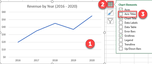
How to Add X and Y Axis Labels in Excel (2 Easy Methods) 2. Using Excel Chart Element Button to Add Axis Labels. In this second method, we will add the X and Y axis labels in Excel by Chart Element Button. In this case, we will label both the horizontal and vertical axis at the same time. The steps are: Steps: Firstly, select the graph. Secondly, click on the Chart Elements option and press Axis Titles.

Excel charts: add title, customize chart axis, legend and ...
How to Add Gridlines in a Chart in Excel? 2 Easy Ways! Click on ' Add Chart Element ' (under the ' Chart Layouts' group). A dropdown menu should appear, with different chart element options. Hover over 'Gridlines'. A submenu consisting of different options relating to gridlines should appear. Select the type of gridlines that you want to add. You can add more than one type of gridlines in your chart.

How to add live total labels to graphs and charts in Excel ...
How to add data labels in excel to graph or chart (Step-by-Step) Add data labels to a chart. 1. Select a data series or a graph. After picking the series, click the data point you want to label. 2. Click Add Chart Element Chart Elements button > Data Labels in the upper right corner, close to the chart. 3. Click the arrow and select an option to modify the location. 4.
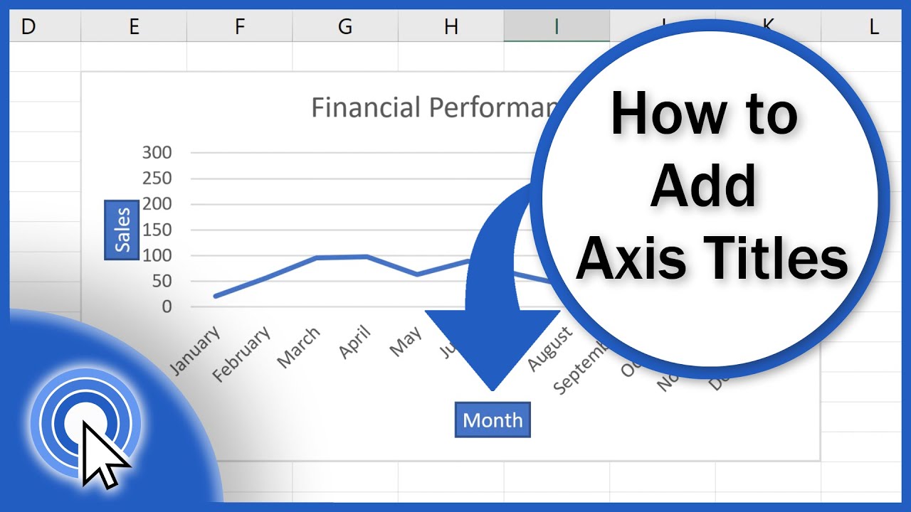
How to Add Axis Titles in Excel
Data Labels in Excel Pivot Chart (Detailed Analysis) Next open Format Data Labels by pressing the More options in the Data Labels. Then on the side panel, click on the Value From Cells. Next, in the dialog box, Select D5:D11, and click OK. Right after clicking OK, you will notice that there are percentage signs showing on top of the columns. 4. Changing Appearance of Pivot Chart Labels

How to add total labels to stacked column chart in Excel?
How to Add Data Labels in Excel - Excelchat | Excelchat After inserting a chart in Excel 2010 and earlier versions we need to do the followings to add data labels to the chart; Click inside the chart area to display the Chart Tools. Figure 2. Chart Tools Click on Layout tab of the Chart Tools. In Labels group, click on Data Labels and select the position to add labels to the chart. Figure 3.

Format Data Labels in Excel- Instructions - TeachUcomp, Inc.
How to Insert Axis Labels In An Excel Chart | Excelchat We will go to Chart Design and select Add Chart Element Figure 6 - Insert axis labels in Excel In the drop-down menu, we will click on Axis Titles, and subsequently, select Primary vertical Figure 7 - Edit vertical axis labels in Excel Now, we can enter the name we want for the primary vertical axis label.

How to add or move data labels in Excel chart?
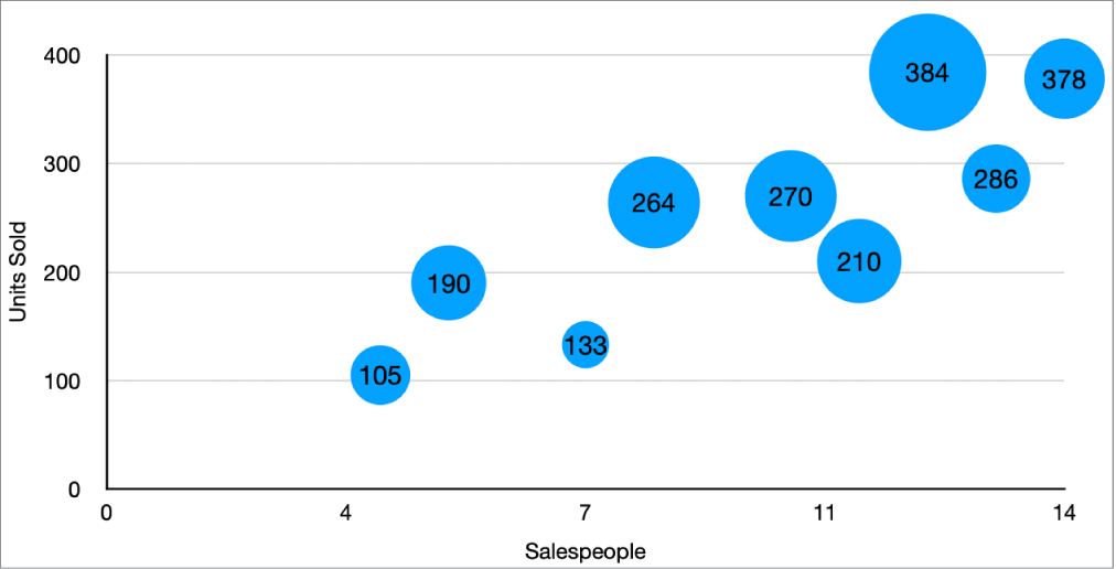
How to Add Labels to Scatterplot Points in Excel - Statology Step 3: Add Labels to Points. Next, click anywhere on the chart until a green plus (+) sign appears in the top right corner. Then click Data Labels, then click More Options…. In the Format Data Labels window that appears on the right of the screen, uncheck the box next to Y Value and check the box next to Value From Cells.

Two-Level Axis Labels (Microsoft Excel)
How to add data labels from different column in an Excel chart? Right click the data series in the chart, and select Add Data Labels > Add Data Labels from the context menu to add data labels. 2. Click any data label to select all data labels, and then click the specified data label to select it only in the chart. 3.

How to Add Two Data Labels in Excel Chart (with Easy Steps ...
Add data labels and callouts to charts in Excel 365 - EasyTweaks.com The steps that I will share in this guide apply to Excel 2021 / 2019 / 2016. Step #1: After generating the chart in Excel, right-click anywhere within the chart and select Add labels . Note that you can also select the very handy option of Adding data Callouts.

Add label to Excel chart line • AuditExcel.co.za MS Excel ...
How to Add Axis Labels in Excel Charts - Step-by-Step (2022) - Spreadsheeto How to add axis titles 1. Left-click the Excel chart. 2. Click the plus button in the upper right corner of the chart. 3. Click Axis Titles to put a checkmark in the axis title checkbox. This will display axis titles. 4. Click the added axis title text box to write your axis label.
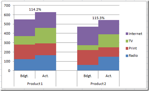
How-to Add Centered Labels Above an Excel Clustered Stacked ...
How to add or move data labels in Excel chart? - ExtendOffice To add or move data labels in a chart, you can do as below steps: In Excel 2013 or 2016. 1. Click the chart to show the Chart Elements button .. 2. Then click the Chart Elements, and check Data Labels, then you can click the arrow to choose an option about the data labels in the sub menu.See screenshot:

Add label to Excel chart line • AuditExcel.co.za MS Excel ...
How to Add Axis Labels to a Chart in Excel | CustomGuide Add Data Labels. Use data labels to label the values of individual chart elements. Select the chart. Click the Chart Elements button. Click the Data Labels check box. In the Chart Elements menu, click the Data Labels list arrow to change the position of the data labels.

Enable or Disable Excel Data Labels at the click of a button ...
Adding Data Labels to Charts/Graphs in Excel First Method - In the Design tab of the Chart Tools contextual tab, go to the Chart Layouts group on the far left side of the ribbon, and click Add Chart Element. In the drop-down menu, hover on Data Labels. This will cause a second drop-down menu to appear. Choose Outside End for now and note how it adds labels to the end of each pie portion.

Change the format of data labels in a chart
Add or remove data labels in a chart - support.microsoft.com This displays the Chart Tools, adding the Design, and Format tabs. Do one of the following: On the Design tab, in the Chart Layouts group, click Add Chart Element, choose Data Labels, and then click None. Click a data label one time to select all data labels in a data series or two times to select just one data label that you want to delete, and then press DELETE. Right-click a data …

Adding rich data labels to charts in Excel 2013 | Microsoft ...
Dynamically Label Excel Chart Series Lines - My Online Training Hub 26.09.2017 · Hi Mynda – thanks for all your columns. You can use the Quick Layout function in Excel (Design tab of the chart) to do the labels to the right of the lines in the chart. Use Quick Layout 6. You may need to swap the columns and rows in your data for it to show. Then you simply modify the labels to show only the series name. I just happened to ...

Directly Labeling Your Line Graphs | Depict Data Studio
Correlation Chart in Excel - GeeksforGeeks Jun 23, 2021 · You can further format the above chart by making it more interactive by changing the “Chart Styles”, adding suitable “Axis Titles”, “Chart Title”, “Data Labels”, changing the “Chart Type” etc. It can be done using the “+” button in the top right corner of the Excel chart.

How to add data labels from different column in an Excel chart?
Add Excel Chart Labels. Adding Chart Labels in Excel. Excel ... - OzGrid With the above data, generate the chart below. First select the chart, then access the dialog below from the Chart Tools for Excel 1.1 toolbar / Charts / Add Labels. You may also access this tool by right-clicking on the chart and selecting Add Labels. The same dialog will appear.
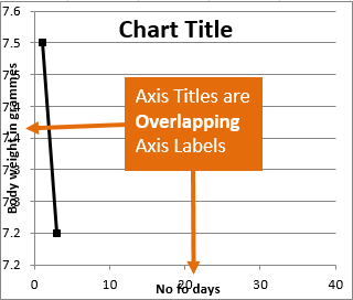
Resize the Plot Area in Excel Chart - Titles and Labels Overlap
Edit titles or data labels in a chart - support.microsoft.com On a chart, click one time or two times on the data label that you want to link to a corresponding worksheet cell. The first click selects the data labels for the whole data series, and the second click selects the individual data label. Right-click the data label, and then click Format Data Label or Format Data Labels.

How to Add Data Labels to your Excel Chart in Excel 2013
How to Create Charts in Excel (In Easy Steps) - Excel Easy To move the legend to the right side of the chart, execute the following steps. 1. Select the chart. 2. Click the + button on the right side of the chart, click the arrow next to Legend and click Right. Result: Data Labels. You can use data labels to focus your readers' attention on a single data series or data point. 1. Select the chart. 2.

Add or remove data labels in a chart

Add Data Labels for Total to Stacked Columns in #Excel | wmfexcel

Chart axes, legend, data labels, trendline in Excel - Tech Funda

Add a Data Callout Label to Charts in Excel 2013 – Software ...
Directly Labeling Excel Charts - PolicyViz

Google Workspace Updates: Get more control over chart data ...

Add data labels and callouts to charts in Excel 365 ...
Change the look of chart text and labels in Numbers on Mac ...

How to Add Two Data Labels in Excel Chart (with Easy Steps ...

Adding rich data labels to charts in Excel 2013 | Microsoft ...

Microsoft Excel Tutorials: Add Data Labels to a Pie Chart
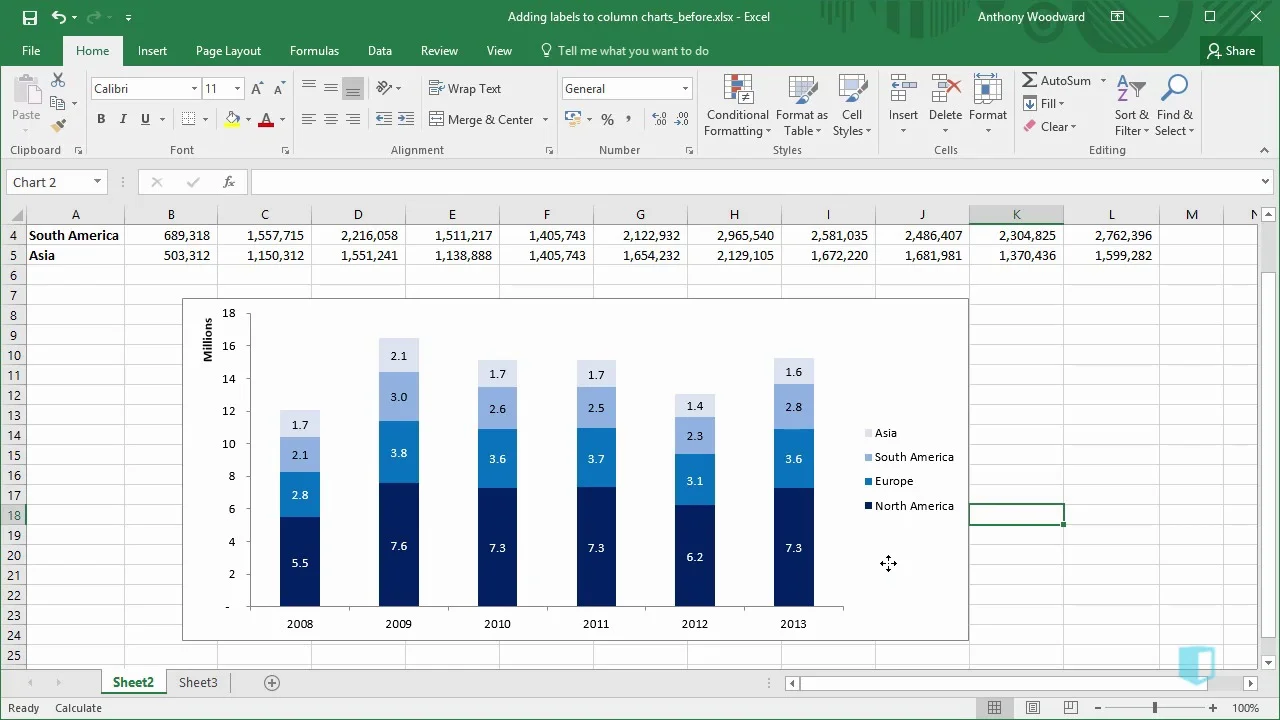
Adding Labels to Column Charts | Online Excel - KPMG Tax - Digital Now Course Training
Excel charts: add title, customize chart axis, legend and ...

Add or remove data labels in a chart

How to Add Data Labels to an Excel 2010 Chart - dummies

Change the format of data labels in a chart

Excel Custom Chart Labels • My Online Training Hub
How to add total labels to stacked column chart in Excel?
Excel Data Labels: How to add totals as labels to a stacked ...
Move and Align Chart Titles, Labels, Legends with the Arrow ...

How to Add Total Data Labels to the Excel Stacked Bar Chart ...
How to add Axis Labels (X & Y) in Excel & Google Sheets ...

Custom data labels in a chart
Post a Comment for "45 adding chart labels in excel"