38 pivot table excel multiple row labels

How to repeat row labels for group in pivot table? - ExtendOffice 1. Click any cell in your pivot table, and click Design under PivotTable Tools tab, and then click Report Layout > Show in Outline Form to display the pivot table as outline form, see screenshots: 2. After expanding the row labels, go on clicking Repeat All Item Labels under Report Layout, see screenshot: 3. › xlpivot08Excel Pivot Table Multiple Consolidation Ranges Jul 10, 2022 · Create Pivot Table from Multiple Sheets. To create a Pivot Table in Microsoft Excel, you can use data from different sheets in a workbook, or from different workbooks. Use one of the following 3 methods - Multiple Consolidation Ranges, Power Query or a Union Query. 1) Multiple Consolidation Ranges

Pivot Table Multiple Row Labels? [SOLVED] - Excel Help Forum Is it possible to have two Row Labels showing in a Pivot Table, instead of one showing as a sub-category of the other. I have a spreadsheet that shows the status (Design, Development, Testing, Live), owner and engineer for software. I currently have to have two separate pivot tables: 1) showing count of software in each status for each owner.

Pivot table excel multiple row labels

Remove PivotTable Duplicate Row Labels - Excel Help Forum Re: Remove PivotTable Duplicate Row Labels. Sometimes when the cells are stored in different formats within the same column in the raw data, they get duplicated. Also, if there is space/s at the beginning or at the end of these fields, when you filter them out they look the same, however, when you plot a Pivot Table, they appear as separate ... › excel-pivot-table-formatHow to Format Excel Pivot Table - Contextures Excel Tips Jun 22, 2022 · Video: Change Pivot Table Labels. Watch this short video tutorial to see how to make these changes to the pivot table headings and labels. Get the Sample File. No Macros: To experiment with pivot table styles and formatting, download the sample file. The zipped file is in xlsx format, and and does NOT contain any macros. en.wikipedia.org › wiki › Pivot_tablePivot table - Wikipedia Pivot tables are not created automatically. For example, in Microsoft Excel one must first select the entire data in the original table and then go to the Insert tab and select "Pivot Table" (or "Pivot Chart"). The user then has the option of either inserting the pivot table into an existing sheet or creating a new sheet to house the pivot table.

Pivot table excel multiple row labels. Automatic Row And Column Pivot Table Labels - How To Excel At Excel Select the data set you want to use for your table The first thing to do is put your cursor somewhere in your data list Select the Insert Tab Hit Pivot Table icon Next select Pivot Table option Select a table or range option Select to put your Table on a New Worksheet or on the current one, for this tutorial select the first option Click Ok Help. How do I do multiple Value Filters on a pivot table row label ... Right-Click on your Row Label > Value Filters... If you have multiple value fields, you should be able to dropdown the listbox under "Show items for which". If you have more than one Row Field make sure that the Value Filter (your field name) title is at the correct level, as you can filter at different levels. Multi-level Pivot Table in Excel - Easy Steps / Become a Pro First, insert a pivot table. Next, drag the following fields to the different areas. 1. Order ID to the Rows area. 2. Amount field to the Values area. 3. Country field and Product field to the Filters area. 4. Next, select United Kingdom from the first filter drop-down and Broccoli from the second filter drop-down. › pivot-tables › compare-listsHow To Compare Multiple Lists of Names with a Pivot Table Jul 08, 2014 · Column E of the Pivot Table contains the Grand Total (sum of columns B:D). People that volunteered all three years will have a “3” in column E. We should sort the pivot table so all the people with a “3” in column E appear at the top of the list. This will make it easier to find the names.

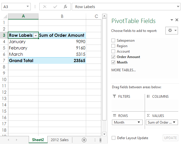
› pivot-table-tips-and-tricks101 Advanced Pivot Table Tips And Tricks You Need To Know Apr 25, 2022 · As a new pivot table user I LOVE this website – very well written! I do have a unique issue I’m hoping to get assistance with. I have a pivot table built out with multiple rows and columns pertaining to new hire information. My boss likes the option to “drill down” and view the source data. Repeat item labels in a PivotTable - support.microsoft.com Right-click the row or column label you want to repeat, and click Field Settings. Click the Layout & Printtab, and check the Repeat item labelsbox. Make sure Show item labels in tabular formis selected. Notes: When you edit any of the repeated labels, the changes you make are applied to all other cells with the same label. Pivot Table Row Labels - Microsoft Community If you go to PivotTable Tools > Analyze > Layout > Report Layout > Show in Tabular Form, your column headers will be used for the row labels. Every once in a while there's a sudden gust of gravity... Report abuse 1 person found this reply helpful · Was this reply helpful? Yes No A. User Replied on December 19, 2017 How to make row labels on same line in pivot table? Make row labels on same line with PivotTable Options You can also go to the PivotTable Options dialog box to set an option to finish this operation. 1. Click any one cell in the pivot table, and right click to choose PivotTable Options, see screenshot: 2.

row - Excel pivot table: How to transpose multiple value in column to a ... Here's the pivot table I have in excel: I have a list of website with their emails address. Sometime you have one email per website, sometime you have 3 emails per website. I want to transpose the multiple emails I have for one website that are in column Email 1 into multiple field such as Email 1, Email 2, Email 3 for EACH corresponding websites. Pivot table row labels in separate columns • AuditExcel.co.za So when you click in the Pivot Table and click on the DESIGN tab one of the options is the Report Layout. Click on this and change it to Tabular form. Your pivot table report will now look like the bottom picture and will be easier to use in other areas of the spreadsheet and in our opinion is also easier to read. Who wants to be a ... How to repeat row labels for group in pivot table? - ExtendOffice Except repeating the row labels for the entire pivot table, you can also apply the feature to a specific field in the pivot table only. 1. Firstly, you need to expand the row labels as outline form as above steps shows, and click one row label which you want to repeat in your pivot table. 2. How to Filter Multiple Values in Pivot Table - Excel Tutorials We will now create our Pivot Table by selecting the range A1:G28 and going to Insert >> Tables >> Pivot Table. On a pop-up that appears, we will simply click OK and our Pivot Table will be created in the new sheet: We will insert our players into the Rows fields, and the sum of points, the sum of rebounds, and the sum of assists into values.

Excel pivot table categorical variables the same in multiple columns (histogram) - Super User

Pivot table row labels side by side - Excel Tutorials You can copy the following table and paste it into your worksheet as Match Destination Formatting. Now, let's create a pivot table ( Insert >> Tables >> Pivot Table) and check all the values in Pivot Table Fields. Fields should look like this. Right-click inside a pivot table and choose PivotTable Options…. Check data as shown on the image below.

Excel Pivot Table Report - Sort Data in Row & Column Labels & in Values Area, use Custom Lists

Multiple row labels on one row in Pivot table | MrExcel Message Board I figured it out - Right click on your pivot table and choose pivot table options/display. Click on "Classic PivotTable layout" Then click on where it is subtotaling your row label and uncheck the subtotal option. D dudeshane0 New Member Joined Oct 23, 2014 Messages 1 Jan 19, 2015 #6 Gerald Higgins said:

EXCEL: SETTING PIVOT TABLE DEFAULTS - Strategic Finance

› documents › excelHow to reverse a pivot table in Excel? - ExtendOffice 5. Now a new pivot table is created, and double click last cell at the right down corner of new Pivot table, then a new table is created in a new worksheet. See screenshots: iv> 6. Then create a new pivot table based on this new table. Select the whole new table, and click Insert > PivotTable > PivotTable. 7.

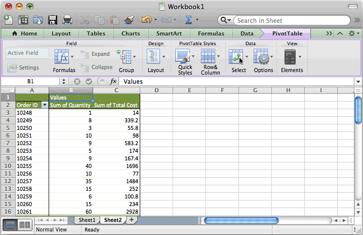
MS Excel 2011 for Mac: Display the fields in the Values Section in multiple columns in a pivot table

How to rename group or row labels in Excel PivotTable? 1. Click at the PivotTable, then click Analyze tab and go to the Active Field textbox. 2. Now in the Active Field textbox, the active field name is displayed, you can change it in the textbox. You can change other Row Labels name by clicking the relative fields in the PivotTable, then rename it in the Active Field textbox.

33 Pivot Table Blank Row Label - Labels Database 2020

Pivot Table Row Labels In the Same Line - Beat Excel! Lets see how to do it. First make a pivot table with required fields. Arrange the fields as shown in left picture. Your initial table will look like right picture. Now click on "Error Code" and access field settings. First check "None" option in "Subtotals & Filters" tab to disable totals after every row.

Pivot Table Excel 2013 | Decorations I Can Make

powerspreadsheets.com › excel-pivot-table-groupExcel Pivot Table Group: Step-By-Step Tutorial To Group Or ... In fact, as mentioned in Excel 2016 Pivot Table Data Crunching: Each time you create a new pivot table in Excel 2016, Excel automatically shares the pivot cache. Pivot Cache sharing has several benefits. Most notably, as I mention above, it reduces memory requirements and file size vs. the scenario where the Pivot Cache isn't shared.

Share :