44 excel 2013 data labels
"Chart created in Excel 2013 is now showing data label values when ... Hello everybody, 1) I created a customized column chart in Excel (A->G/57->83): The data labels show "Name" "%fraction" "(absolute share)" 2) The data of this chart is in the same excel sheet - but "far away" from the chart (AG->AV/444->454) 3) The chart is connected with the data by the "Value from cells" option: If you "right click2 on one of the data labels of the chart -> Click "Format ... Edit titles or data labels in a chart To reposition all data labels for an entire data series, click a data label once to select the data series. To reposition a specific data label, click that data label twice to select it. This displays the Chart Tools , adding the Design , Layout , and Format tabs.
How to Print Labels from Excel - Lifewire To label legends in Excel, select a blank area of the chart. In the upper-right, select the Plus ( +) > check the Legend checkbox. Then, select the cell containing the legend and enter a new name. How do I label a series in Excel? To label a series in Excel, right-click the chart with data series > Select Data.
Excel 2013 data labels
› charts › dynamic-chart-dataCreate Dynamic Chart Data Labels with Slicers - Excel Campus Feb 10, 2016 · Typically a chart will display data labels based on the underlying source data for the chart. In Excel 2013 a new feature called “Value from Cells” was introduced. This feature allows us to specify the a range that we want to use for the labels. Since our data labels will change between a currency ($) and percentage (%) formats, we need a ... How to Format Data and Cells in Microsoft Excel 2013 Changing the font color is as simple as changing the font. By default, your text in Excel 2013 appears in a black font. If you want to change the font color, look for the uppercase A with a colored bar under it in the Font group as pictured below. Select your text, then click on the button to choose the color you want to apply to the selected text. Adding Data Labels to Your Chart (Microsoft Excel) To add data labels in Excel 2013 or Excel 2016, follow these steps: Activate the chart by clicking on it, if necessary. Make sure the Design tab of the ribbon is displayed. (This will appear when the chart is selected.) Click the Add Chart Element drop-down list. Select the Data Labels tool.
Excel 2013 data labels. Excel Charts - Aesthetic Data Labels - Tutorials Point Step 3 − Format the data label choosing the options you want. Make sure that only one data label is selected while formatting. Clone Current Label. To clone the data label created, follow the steps given −. Step 1 − In the Format Data Labels pane, click the Label Options icon. Step 2 − Under Data Label Series, click Clone Current Label ... Move data labels - support.microsoft.com Click any data label once to select all of them, or double-click a specific data label you want to move. Right-click the selection > Chart Elements > Data Labels arrow, and select the placement option you want. Different options are available for different chart types. Creating a chart with dynamic labels - Microsoft Excel 2013 Excel 2013 365 2016. This tip shows how to create dynamically updated chart labels that depend on value or other cells. ... For all labels: on the Format Data Labels task pane, in the Label Options, in the Label Contains group, check Value From Cells and then choose cells: Introduction to the Data Model and Relationships in Excel 2013 ... In Excel, go to the DATA tab and select "From Other Sources", "From Windows Azure Marketplace". Fill out the information with what you have saved from the website: Select that table. Hit "Finish" and then select "Only Create Connection": Note: Some of you might be wondering why I chose "Only Create Connection".
mgconsulting.wordpress.com › 2013/12/09 › add-a-dataAdd a Data Callout Label to Charts in Excel 2013 Dec 09, 2013 · The new Data Callout Labels make it easier to show the details about the data series or its individual data points in a clear and easy to read format. How to Add a Data Callout Label. Click on the data series or chart. In the upper right corner, next to your chart, click the Chart Elements button (plus sign), and then click Data Labels. support.microsoft.com › en-us › officeTutorial: Import Data into Excel, and Create a Data Model However, the same data modeling and Power Pivot features introduced in Excel 2013 also apply to Excel 2016. In these tutorials you learn how to import and explore data in Excel, build and refine a data model using Power Pivot, and create interactive reports with Power View that you can publish, protect, and share. Add or remove data labels in a chart - Microsoft Support To label one data point, after clicking the series, click that data point. In the upper right corner, next to the chart, click Add Chart Element > Data Labels. To change the location, click the arrow, and choose an option. If you want to show your data label inside a text bubble shape, click Data Callout. Adding rich data labels to charts in Excel 2013 - Microsoft 365 Blog You can do this by adjusting the zoom control on the bottom right corner of Excel's chrome. Then, select the value in the data label and hit the right-arrow key on your keyboard. The story behind the data in our example is that the temperature increased significantly on Wednesday and that appeared to help drive up business at the lemonade stand.
Excel 2013 Chart Labels don't appear properly - Microsoft Community You've stumbled on a big problem - Excel 2013 lets you edit data labels directly, but this feature (rich text data labels) is not backwards-compatible and there's no way to turn it off. It's great to be able to modify the text of labels, or direct them to get contents from a worksheet cell. How to create Custom Data Labels in Excel Charts Create the chart as usual. Add default data labels. Click on each unwanted label (using slow double click) and delete it. Select each item where you want the custom label one at a time. Press F2 to move focus to the Formula editing box. Type the equal to sign. Now click on the cell which contains the appropriate label. Change the format of data labels in a chart To get there, after adding your data labels, select the data label to format, and then click Chart Elements > Data Labels > More Options. To go to the appropriate area, click one of the four icons ( Fill & Line, Effects, Size & Properties ( Layout & Properties in Outlook or Word), or Label Options) shown here. Values From Cell: Missing Data Labels Option in Excel 2013? 8. May 27, 2015. #1. Ive inherited a Powerpoin with an embedded Excel chart and data sheet. The graph in Powerpoint shows several instances of a value [CellRange]. Im trying to figure out where its "trying" to pull its data from and I think because the data is not in a contiguous range its having trouble. A couple articles refer to formatting ...
Making a scatter plot in Excel Mac 2011 - YouTube
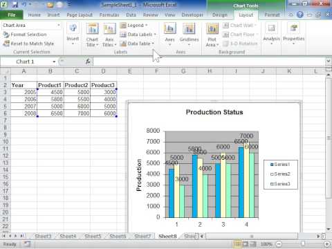
How to Customize Chart Elements in Excel 2013 - dummies To add data labels to your selected chart and position them, click the Chart Elements button next to the chart and then select the Data Labels check box before you select one of the following options on its continuation menu: Center to position the data labels in the middle of each data point. Inside End to position the data labels inside each ...

Excel 3-D Pie Charts
Apply Custom Data Labels to Charted Points - Peltier Tech For data labels, the best tool by far is the XY chart label add in. I have Excel 2013 and have found that the Excel linked labels are not as reliable when the cells change as Rob Bovey's add in. Excel is complicated enough. We don't need to add complexity. Cheers,

Excel Help: Enable Developer tab in Excel 2010
How to Data Labels in a Line Graph in Excel 2013 - YouTube Want to insert Data Labels in a line graph in Microsoft® Excel 2013? Follow the easy steps shown in this video. Content in this video is provided on an ""as ...

MS Excel 2010 / How to display data labels on the chart - YouTube
How to add data labels from different column in an Excel chart? Right click the data series in the chart, and select Add Data Labels > Add Data Labels from the context menu to add data labels. 2. Click any data label to select all data labels, and then click the specified data label to select it only in the chart. 3.

Chapter 3 Excel 2007/2010 Charts
› format-data-labels-in-excelFormat Data Labels in Excel- Instructions - TeachUcomp, Inc. Nov 14, 2019 · Then select the “Format Data Labels…” command from the pop-up menu that appears to format data labels in Excel. Using either method then displays the “Format Data Labels” task pane at the right side of the screen. Format Data Labels in Excel- Instructions: A picture of the “Format Data Labels” task pane in Excel.

How to Add Data Labels in Excel - Excelchat | Excelchat
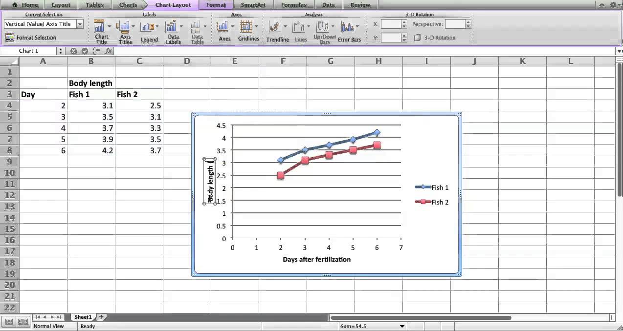
Excel Tips n Tricks -Tip 8 (Applying Chart Data Labels From a Range in ... Click on the plus symbol, the first icon, and check "Data Labels". Now you will see them added to your chart. You can also click on the right arrow on "Data Labels" and select where you want the data labels to be aligned, in other words center, right, top, bottom and so on. Picture 4 4. I modified the chart and axis titles to look good.

Excel 2013 Tutorial Formatting Data Labels Microsoft Training Lesson 28.6 - YouTube
How to Add Data Labels to your Excel Chart in Excel 2013 Data labels show the values next to the corresponding chart element, for instance a percentage next to a piece from a pie chart, or a total value next to a column in a column chart. You can choose...

Enable or Disable Excel Data Labels at the click of a button - How To - PakAccountants.com
Quick Tip: Excel 2013 offers flexible data labels | TechRepublic right-click and choose Insert Data Label Field. In the next dialog, select [Cell] Choose Cell. When Excel displays the source dialog, click the cell that contains the MIN () function, and click OK....
Format Number Options for Chart Data Labels in Excel 2011 for Mac
How to Add Data Labels in Excel - Excelchat | Excelchat In Excel 2013 and the later versions we need to do the followings; Click anywhere in the chart area to display the Chart Elements button Figure 5. Chart Elements Button Click the Chart Elements button > Select the Data Labels, then click the Arrow to choose the data labels position. Figure 6. How to Add Data Labels in Excel 2013 Figure 7.

Excel Treemap - Beat Excel!
› excel › how-to-add-total-dataHow to Add Total Data Labels to the Excel Stacked Bar Chart Apr 03, 2013 · Step 4: Right click your new line chart and select “Add Data Labels” Step 5: Right click your new data labels and format them so that their label position is “Above”; also make the labels bold and increase the font size. Step 6: Right click the line, select “Format Data Series”; in the Line Color menu, select “No line”

How to format data labels in excel charts and data elements - YouTube
Excel Data Labels - Value from Cells I created a chart and linked the data labels to a series of cells, as 2013 allows in Value From Cells option. I pre-select e.g. 100 data rows even though it initially contains values in 10 of them. When I reopen the workbook and add x and y value and a new label (where I left empty cells to do so) that data point 'icon' comes on to the graph ...
Excel 2010 Remove Data Labels from a Chart - YouTube
How to hide zero data labels in chart in Excel? - ExtendOffice Note: In Excel 2013, you can right click the any data label and select Format Data Labels to open the Format Data Labels pane; then click Number to expand its option; next click the Category box and select the Custom from the drop down list, and type #"" into the Format Code text box, and click the Add button.

How to Add Data Labels in Excel - Excelchat | Excelchat
Data Labels Not Saving - Microsoft Tech Community Data Labels Not Saving I keep making the same edits each and everytime I open the pivot chart I created with excel 2013. Fo some reason the data labels keep disappering.

SQL & BI Learning: Pie Chart with data labels outside in ssrs
› excel_barcodeExcel Barcode Generator Add-in: Create Barcodes in Excel 2019 ... Office Excel Barcode Encoder Add-In is a reliable, efficient and convenient barcode generator for Microsoft Excel 2016/2013/2010/2007, which is designed for office users to embed most popular barcodes into Excel workbooks. It is widely applied in many industries.

Enable or Disable Excel Data Labels at the click of a button - How To - PakAccountants.com in ...
chandoo.org › wp › change-data-labels-in-chartsHow to Change Excel Chart Data Labels to Custom Values? May 05, 2010 · Now, click on any data label. This will select “all” data labels. Now click once again. At this point excel will select only one data label. Go to Formula bar, press = and point to the cell where the data label for that chart data point is defined. Repeat the process for all other data labels, one after another. See the screencast.
ExcelMadeEasy: Vba add legend to chart in Excel
Values From Cell: Missing Data Labels Option in Excel 2013? When a chart created in 2013 using the "Values from Cell" data label option is opened with any earlier version of Excel, the data labels will show as " [CELLRANGE]". If you want to ensure that data labels survive different generations of Excel, you need to revert to the old technique: Insert data labels Edit each individual data label

Excel pivot filter – How to filter data in a pivot table
Adding Data Labels to Your Chart (Microsoft Excel) To add data labels in Excel 2013 or Excel 2016, follow these steps: Activate the chart by clicking on it, if necessary. Make sure the Design tab of the ribbon is displayed. (This will appear when the chart is selected.) Click the Add Chart Element drop-down list. Select the Data Labels tool.

32 How To Label A Pie Chart In Excel - Labels Information List
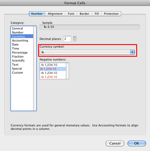
How to Format Data and Cells in Microsoft Excel 2013 Changing the font color is as simple as changing the font. By default, your text in Excel 2013 appears in a black font. If you want to change the font color, look for the uppercase A with a colored bar under it in the Font group as pictured below. Select your text, then click on the button to choose the color you want to apply to the selected text.
Post a Comment for "44 excel 2013 data labels"