40 excel graph data labels

How to Add Labels to Scatterplot Points in Excel - Statology Step 3: Add Labels to Points. Next, click anywhere on the chart until a green plus (+) sign appears in the top right corner. Then click Data Labels, then click More Options… In the Format Data Labels window that appears on the right of the screen, uncheck the box next to Y Value and check the box next to Value From Cells. How To Use Dynamic Data Labels To Create Interactive Excel Charts To create a column chart with dynamic data labels, you need to follow these given steps. Select the data & Create a Combo Chart. Now select the column chart for revenue data and a line chart with marker for data labels Add Data Labels to the Line Chart With Marker. After then remove the Line Color and Marker Color.

Prevent Overlapping Data Labels in Excel Charts - Peltier Tech Apply Data Labels to Charts on Active Sheet, and Correct Overlaps Can be called using Alt+F8 ApplySlopeChartDataLabelsToChart (cht As Chart) Apply Data Labels to Chart cht Called by other code, e.g., ApplySlopeChartDataLabelsToActiveChart FixTheseLabels (cht As Chart, iPoint As Long, LabelPosition As XlDataLabelPosition)

Excel graph data labels

Excel charts: add title, customize chart axis, legend and data labels ... Click the Chart Elements button, and select the Data Labels option. For example, this is how we can add labels to one of the data series in our Excel chart: For specific chart types, such as pie chart, you can also choose the labels location. For this, click the arrow next to Data Labels, and choose the option you want. Custom Chart Data Labels In Excel With Formulas Follow the steps below to create the custom data labels. Select the chart label you want to change. In the formula-bar hit = (equals), select the cell reference containing your chart label's data. In this case, the first label is in cell E2. Finally, repeat for all your chart laebls. Add a DATA LABEL to ONE POINT on a chart in Excel Click on the chart line to add the data point to. All the data points will be highlighted. Click again on the single point that you want to add a data label to. Right-click and select ' Add data label '. This is the key step! Right-click again on the data point itself (not the label) and select ' Format data label '.

Excel graph data labels. how to add data labels into Excel graphs - storytelling with data You can download the corresponding Excel file to follow along with these steps: Right-click on a point and choose Add Data Label. You can choose any point to add a label—I'm strategically choosing the endpoint because that's where a label would best align with my design. Excel defaults to labeling the numeric value, as shown below. engineerexcel.com › 3-axis-graph-excel3 Axis Graph Excel Method: Add a Third Y-Axis - EngineerExcel By default, Excel adds the y-values of the data series. In this case, these were the scaled values, which wouldn’t have been accurate labels for the axis (they would have corresponded directly to the secondary axis). However, in Excel 2013 and later, you can choose a range for the data labels. For this chart, that is the array of unscaled ... chandoo.org › wp › change-data-labels-in-chartsHow to Change Excel Chart Data Labels to Custom Values? May 05, 2010 · Now, click on any data label. This will select “all” data labels. Now click once again. At this point excel will select only one data label. Go to Formula bar, press = and point to the cell where the data label for that chart data point is defined. Repeat the process for all other data labels, one after another. See the screencast. Excel Charts - Aesthetic Data Labels - Tutorials Point Step 3 − Format the data label choosing the options you want. Make sure that only one data label is selected while formatting. Clone Current Label. To clone the data label created, follow the steps given −. Step 1 − In the Format Data Labels pane, click the Label Options icon. Step 2 − Under Data Label Series, click Clone Current Label ...

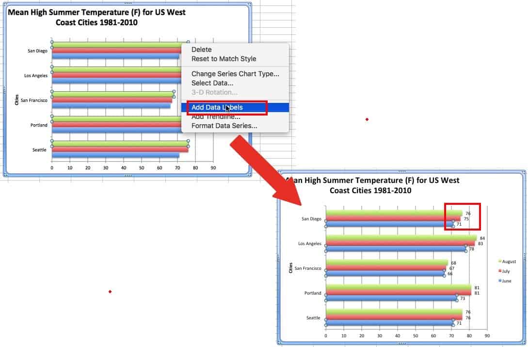
› linking-a-graph-inLinking a graph in PowerPoint to the Excel data so the graph ... Each method starts with you creating the graph in Excel first, because we will be copying the graph created in Excel into the PowerPoint slide. Method 1: Basic Paste. After you have created the graph in Excel, click on it and copy it (press Ctrl+C or click the copy button on the Home ribbon). Switch to your PowerPoint slide. Edit titles or data labels in a chart - support.microsoft.com The first click selects the data labels for the whole data series, and the second click selects the individual data label. Right-click the data label, and then click Format Data Label or Format Data Labels. Click Label Options if it's not selected, and then select the Reset Label Text check box. Top of Page Excel tutorial: How to use data labels Generally, the easiest way to show data labels to use the chart elements menu. When you check the box, you'll see data labels appear in the chart. If you have more than one data series, you can select a series first, then turn on data labels for that series only. You can even select a single bar, and show just one data label. How to add data labels from different column in an Excel chart? This method will guide you to manually add a data label from a cell of different column at a time in an Excel chart. 1. Right click the data series in the chart, and select Add Data Labels > Add Data Labels from the context menu to add data labels. 2. Click any data label to select all data labels, and then click the specified data label to select it only in the chart.

Add / Move Data Labels in Charts - Excel & Google Sheets We'll start with the same dataset that we went over in Excel to review how to add and move data labels to charts. Add and Move Data Labels in Google Sheets. Double Click Chart; Select Customize under Chart Editor; Select Series . 4. Check Data Labels. 5. Select which Position to move the data labels in comparison to the bars. Final Graph with Google Sheets. After moving the dataset to the center, you can see the final graph has the data labels where we want. Creating a chart with dynamic labels - Microsoft Excel 2016 1. Right-click on the chart and in the popup menu, select Add Data Labels and again Add Data Labels : 2. Do one of the following: For all labels: on the Format Data Labels pane, in the Label Options, in the Label Contains group, check Value From Cells and then choose cells: For the specific label: double-click on the label value, in the popup ... How to add or move data labels in Excel chart? - ExtendOffice To add or move data labels in a chart, you can do as below steps: In Excel 2013 or 2016. 1. Click the chart to show the Chart Elements button . 2. Then click the Chart Elements, and check Data Labels, then you can click the arrow to choose an option about the data labels in the sub menu. See screenshot: In Excel 2010 or 2007 Excel: How to Create a Bubble Chart with Labels - Statology This tutorial provides a step-by-step example of how to create the following bubble chart with labels in Excel: Step 1: Enter the Data. First, let's enter the following data into Excel that shows various attributes for 10 different basketball players: Step 2: Create the Bubble Chart. Next, highlight the cells in the range B2:D11.

Excel Charts: Creating Custom Data Labels - YouTube

Excel charts: how to move data labels to legend - Microsoft Tech Community You can't do that, but you can show a data table below the chart instead of data labels: Click anywhere on the chart. On the Design tab of the ribbon (under Chart Tools), in the Chart Layouts group, click Add Chart Element > Data Table > With Legend Keys (or No Legend Keys if you prefer)

32 What Is A Data Label In Excel - Labels Design Ideas 2020

› make-graph-excel-chart-templateHow to create a chart (graph) in Excel and save it as template Oct 22, 2015 · Simply select the data to be included in the graph and press one of the following shortcuts: Alt + F1 to insert the default chart in the current worksheet. F11 to create the default chart in a new sheet. How to change the default chart type in Excel. When you make a graph in Excel, the default chart format is a two-dimensional column chart.

How to Make a Bar Chart in Excel | Smartsheet

› charts › dynamic-chart-dataCreate Dynamic Chart Data Labels with Slicers - Excel Campus Feb 10, 2016 · Step 3: Use the TEXT Function to Format the Labels. Typically a chart will display data labels based on the underlying source data for the chart. In Excel 2013 a new feature called “Value from Cells” was introduced. This feature allows us to specify the a range that we want to use for the labels.

Creating a chart with dynamic labels - Microsoft Excel 2016

Add data labels and callouts to charts in Excel 365 - EasyTweaks.com Step #1: After generating the chart in Excel, right-click anywhere within the chart and select Add labels . Note that you can also select the very handy option of Adding data Callouts. Step #2: When you select the "Add Labels" option, all the different portions of the chart will automatically take on the corresponding values in the table ...

Excel Chart Elements: Parts of Charts in Excel | ExcelDemy

› data-series-data-points-dataUnderstanding Excel Chart Data Series, Data Points, and Data ... When a chart is selected, the Chart Tools appears in the ribbon and contains two tabs. The Format tab and the Design tab. Select Shape Fill to open the Fill Colors menu. In the Standard Colors section, choose the color you wish to apply. Highlight Data with an Exploding Pie Chart Individual slices of a pie chart are usually different colors.

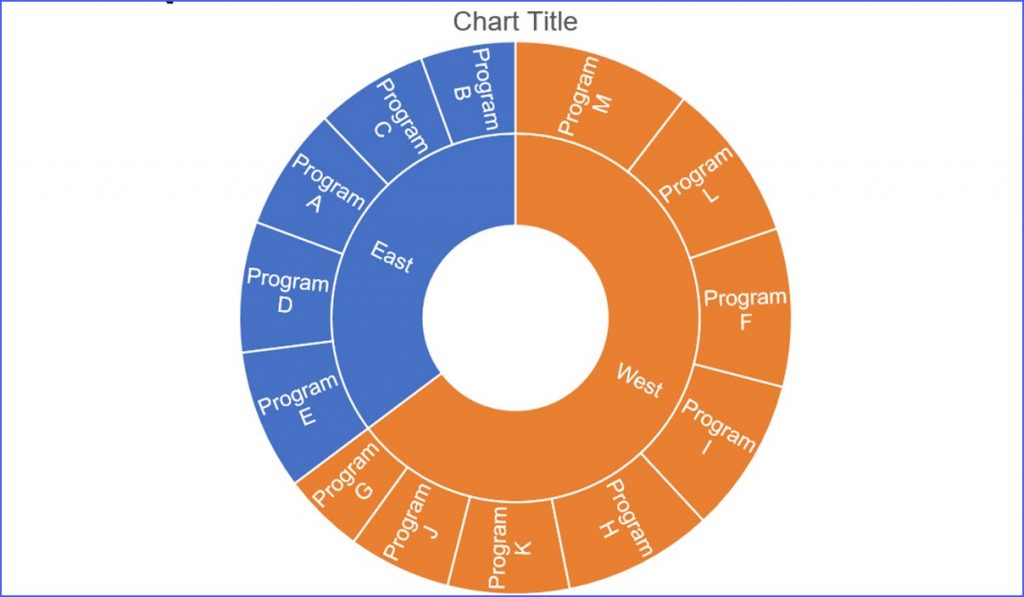
How to Make a Sunburst Chart - ExcelNotes

How to I rotate data labels on a column chart so that they are ... To change the text direction, first of all, please double click on the data label and make sure the data are selected (with a box surrounded like following image). Then on your right panel, the Format Data Labels panel should be opened. Go to Text Options > Text Box > Text direction > Rotate. And the text direction in the labels should be in ...

MEDIAN Don Steward mathematics teaching: comparing two data sets

How to Create a Bar Chart With Labels Inside Bars in Excel In the chart, right-click the Series "# Footballers" Data Labels and then, on the short-cut menu, click Format Data Labels. 8. In the Format Data Labels pane, under Label Options selected, set the Label Position to Inside End. 9. Next, in the chart, select the Series 2 Data Labels and then set the Label Position to Inside Base. 10.

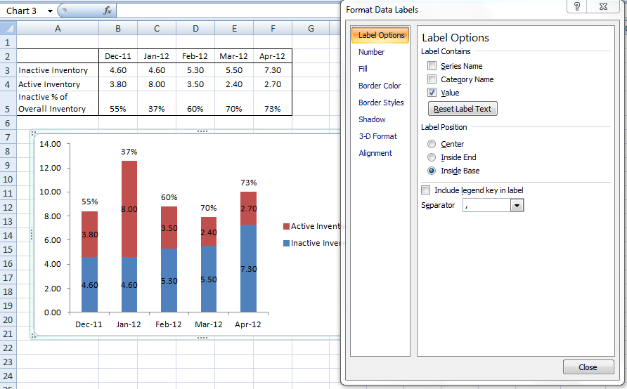
Data label in the graph not showing percentage option. only value ... Normally when you put a data label onto a graph, it gives you the option to insert values as numbers or percentages. In the current graph, which I am developing, the percentage option not showing. Enclosed is the screenshot. Can anyone help me to bring the percentage option as well in this graph data label? Thanks & Regards, Dipil Labels: Excel

Excel Course: Inserting Graphs

› office-addins-blog › 2018/10/10Find, label and highlight a certain data point in Excel ... Oct 10, 2018 · Select the Data Labels box and choose where to position the label. By default, Excel shows one numeric value for the label, y value in our case. To display both x and y values, right-click the label, click Format Data Labels…, select the X Value and Y value boxes, and set the Separator of your choosing: Label the data point by name

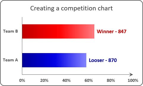
Custom Data Labels with Colors and Symbols in Excel Charts – [How To] - KING OF EXCEL

How to Place Labels Directly Through Your Line Graph in Microsoft Excel Right-click on top of one of those circular data points. You'll see a pop-up window. Click on Add Data Labels. Your unformatted labels will appear to the right of each data point: Click just once on any of those data labels. You'll see little squares around each data point. Then, right-click on any of those data labels.

charts - Excel, giving data labels to only the top/bottom X% values - Stack Overflow

Format Data Labels in Excel- Instructions - TeachUcomp, Inc. To format data labels in Excel, choose the set of data labels to format. To do this, click the "Format" tab within the "Chart Tools" contextual tab in the Ribbon. Then select the data labels to format from the "Chart Elements" drop-down in the "Current Selection" button group. Then click the "Format Selection" button that ...

Show Trend Arrows in Excel Chart Data Labels

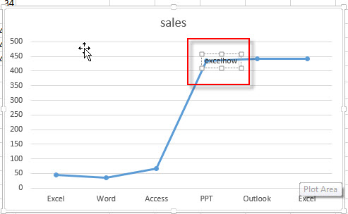
How to create Custom Data Labels in Excel Charts Add data labels Create a simple line chart while selecting the first two columns only. Now Add Regular Data Labels. Two ways to do it. Click on the Plus sign next to the chart and choose the Data Labels option. We do NOT want the data to be shown. To customize it, click on the arrow next to Data Labels and choose More Options …

How-to Put Percentage Labels on Top of a Stacked Column Chart - Excel Dashboard Templates

Add or remove data labels in a chart - support.microsoft.com Add data labels to a chart Click the data series or chart. To label one data point, after clicking the series, click that data point. In the upper right corner, next to the chart, click Add Chart Element > Data Labels. To change the location, click the arrow, and choose an option. If you want to ...

Triangle Graph Paper | Equilateral Triangle Graph Paper

How to Use Cell Values for Excel Chart Labels Select the chart, choose the "Chart Elements" option, click the "Data Labels" arrow, and then "More Options." Uncheck the "Value" box and check the "Value From Cells" box. Select cells C2:C6 to use for the data label range and then click the "OK" button. The values from these cells are now used for the chart data labels.

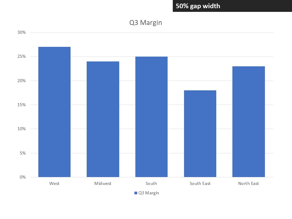
7 Steps to make a professional looking column graph in Excel or PowerPoint | Think Outside The Slide

Add a DATA LABEL to ONE POINT on a chart in Excel Click on the chart line to add the data point to. All the data points will be highlighted. Click again on the single point that you want to add a data label to. Right-click and select ' Add data label '. This is the key step! Right-click again on the data point itself (not the label) and select ' Format data label '.

31 What Is A Label In Excel - Labels For Your Ideas

Custom Chart Data Labels In Excel With Formulas Follow the steps below to create the custom data labels. Select the chart label you want to change. In the formula-bar hit = (equals), select the cell reference containing your chart label's data. In this case, the first label is in cell E2. Finally, repeat for all your chart laebls.

How to Make a Graph in Google Sheets (Scatter Plot) - YouTube

Excel charts: add title, customize chart axis, legend and data labels ... Click the Chart Elements button, and select the Data Labels option. For example, this is how we can add labels to one of the data series in our Excel chart: For specific chart types, such as pie chart, you can also choose the labels location. For this, click the arrow next to Data Labels, and choose the option you want.

Share :