44 excel chart data labels in millions

Formatting axis labels on a paginated report chart ... Right-click the axis you want to format and click Axis Properties to change values for the axis text, numeric and date formats, major and minor tick marks, auto-fitting for labels, and the thickness, color, and style of the axis line. To change values for the axis title, right-click the axis title, and click Axis Title Properties. How to insert a toggle in Excel Inserting a toggle button. Once the Developer tab is visible, you can find the Button command under the Insert button in the Controls section.When you click the Insert button, you will see the Toggle Button command under the ActiveX Controls section.. Clicking the Toggle Button changes the cursor into a plus. Click anywhere to insert a default toggle button, or hold and drag the cursor to ...

Solved: Display Unit Formatting - Microsoft ... - Power BI I am wondering if it is possible to correct the current formatting of display units in Power BI. Currently, I have a report which displays values both in the millions and in the billions, and the Display Units are set to auto on both cards and a bar chart. However, the unit abbreviations displayed are : bn = billions. M = millions.

Excel chart data labels in millions

How to create a map chart - Get Digital Help How to insert a map chart Select data (A1:B56) Go to tab "Insert" on the ribbon Press with left mouse button on the "Maps" icon This world map shows up, US states are barely visible. This is not what we want. Back to top 3. Map Chart settings Double press with the left mouse button on the map to access chart formatting, see the image below. › ms-excel › analyzing-50Analyzing 50 million records in Excel - Master Data Analysis Jul 31, 2016 · Step 3: Load the data into the Power Pivot Data Model. After removing the headers, you just need to load the data into the Power Pivot Data Model. To do this go to File Close & Load To… On the ‘Load To’ dialog box, select ‘Only Create Connection’, then click on the checkbox ‘Add this data to the Data Model’ and click on Load. › charts › actual-vs-target-chartActual vs Targets Chart in Excel - Excel Campus Nov 04, 2019 · You can change the order of the data in your chart by choosing Select Data on the Chart Design tab on the Ribbon. Converting a Column Chart to a Bar Chart . Changing your chart to to a bar graph is actually really easy. With the chart selected, go to the Chart Design tab on the Ribbon, and then select Change Chart Type.

Excel chart data labels in millions. How to round your data in k $ without formula with Excel? In Excel, you can easily display your numbers in kilo dollars K$ or million dollars (M$) with 3 methods. In this article you will find 3 techniques to display a result in K$ (or m$ for the millions]. Each technique have their own benefits and disadvantages. MsoChartElementType enumeration (Office) | Microsoft Docs Display data label as a callout. msoElementDataLabelCenter: 202: Display data label in center. msoElementDataLabelInsideBase: 204: Display data label inside at the base. msoElementDataLabelInsideEnd: 203: Display data label inside at the end. msoElementDataLabelLeft: 206: Display data label to the left. msoElementDataLabelNone: 200: Do not ... › skip-dates-in-excelSkip Dates in Excel Chart Axis - myonlinetraininghub.com Jan 28, 2015 · An aside: notice how the vertical axis on the column chart starts at zero but the line chart starts at 146?That’s a visualisation rule – column charts must always start at zero because we subconsciously compare the height of the columns and so starting at anything but zero can give a misleading impression, whereas the points in the line chart are compared to the axis scale. How to Change the Y Axis in Excel - Alphr Click the dropdown next to "Display Units," then make your selection such as "millions" or "hundreds." To label the displayed units, go to the "Axis Options -> Display units" section. Add a...

Custom Excel number format - Ablebits To create a custom Excel format, open the workbook in which you want to apply and store your format, and follow these steps: Select a cell for which you want to create custom formatting, and press Ctrl+1 to open the Format Cells dialog. Under Category, select Custom. Type the format code in the Type box. Click OK to save the newly created format. › charts › axis-labelsHow to add Axis Labels (X & Y) in Excel & Google Sheets ... Excel offers several different charts and graphs to show your data. In this example, we are going to show a line graph that shows revenue for a company over a five-year period. In the below example, you can see how essential labels are because in this below graph, the user would have trouble understanding the amount of revenue over this period. How to Make a Frequency Distribution Table & Graph in Excel? In addition, I have created an Excel Template [I named it FreqGen] to make the frequency distribution table automatically. Just input data in the template and get the frequency distribution table automatically. Except for these 7 methods, if you know any other techniques, let me know in the comment section. Formatting data points on a paginated report chart ... For all chart types, you can show data point labels when you right-click the chart and select Show Data Labels. The position of the data point labels is specified depending on the chart type: On a bar chart, you can reposition the data point label using the BarLabelStyle custom attribute.

How to Add a Trendline in Excel Charts | Upwork Let's look at the steps to add a trendline to your chart in Excel. Select the chart Click the Chart Design tab Click Add Chart Element Select Trendline Select the type of trendline In our example, we'll add a trendline to our graph depicting the average monthly temperatures for Texas. How to format bar charts in Excel — storytelling with data 3. Click on any data label to highlight them all, then right-click and choose Format Data Labels: 4. In the Format Data Labels menu, select Label Options, and in the Label Positions section, choose Inside End. (While you're at it, in the Label Contains section, uncheck "Show Leader Lines." These are almost never necessary.) Images, Charts, Objects Missing in Excel? How to Get Them ... Reason 1: How to get images and charts back if you have deleted them. If you are sure that you have not accidentally deleted charts or images, just scroll down to reason number 2. If you have deleted pictures, charts or objects, try these things: Undo (Ctrl + Z) until pictures are shown. If you have already changed many things, you can repeat ... How to make a scatter plot in Excel - Ablebits Tick off the Data Labels box, click the little black arrow next to it, and then click More Options… On the Format Data Labels pane, switch to the Label Options tab (the last one), and configure your data labels in this way: Select the Value From Cells box, and then select the range from which you want to pull data labels (B2:B6 in our case).

Format Number Options for Chart Data Labels in Excel 2011 for Mac

Format Chart Axis in Excel - Axis Options (Format Axis ... However, In this blog, we will be working with Axis options, Tick marks, Labels, Number > Axis options> Axis options> Format Axis Pane. Axis Options: Axis Options There are multiple options So we will perform one by one. Changing Maximum and Minimum Bounds The first option is to adjust the maximum and minimum bounds for the axis.

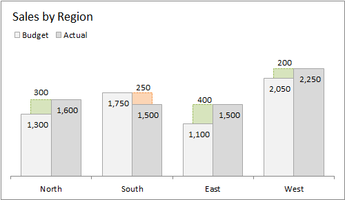
Actual vs Budget or Target Chart in Excel - Variance on Clustered Column or Bar Chart

Create Charts in Excel: Free Excel Video Tutorial The Category Axis identifies the data in the chart. Here, it's telling us which states are included. Pie charts have and usually need Data Labels, which identify what the slices represent. These work in conjunction with or can replace a legend. You'll still want to include a title, though.

Bar-Line Chart with Secondary Axis or Two Panels - Peltier Tech Blog

Peltier Tech Excel Charts and Programming Blog Good Chart Data is in Columns. Excel charts can work with data in columns or in rows. You can use either arrangement and sometimes one just works better than the other. If a chart's source data has more rows than columns, Excel creates the chart with series in columns. A pivot chart always plots the pivot table with series in columns.

34 What Is An Axis Label - Labels For Your Ideas

Altering the Displayed Format of Numbers to the Nearest ... The first format will round to the nearest thousand, and the second will round to the nearest million. If you are looking for a custom format that will round to some other power of 10, you are out of luck, however.

UWP UI Controls - Syncfusion - Visual Studio Marketplace

Axis.DisplayUnit property (Excel) | Microsoft Docs The unit label can also be one of the following constants: xlCustom or xlNone. Using unit labels when charting large values makes your tick mark labels easier to read. For example, if you label your value axis in units of hundreds, thousands, or millions, you can use smaller numeric values at the tick marks on the axis.

Share :